Merging and Joining

Reading Week

Sometimes, we will want to combine data from different sources about the same subject - perhaps we want to compare the GDP in a country with life expectancy, or the proportion of free schools meals with the level of unemployment.

Aims

• Understand joins
• Work with joining dataframes in Pandas
• Create your own examples

Downloading the Data

Let’s grab the data we will need this week from our course website and save it into our data folder. If you’ve not already created a data folder then do so using the following command.

Don’t worry if it generates an error, that means you’ve already got a data folder.

!mkdir data

mkdir: cannot create directory ‘data’: File exists

!mkdir data/wk5
!curl https://s3.eu-west-2.amazonaws.com/qm2/wk3/UN_Life_all.csv -o ./data/wk5/UN_Life_all.csv
!curl https://s3.eu-west-2.amazonaws.com/qm2/wk3/UN_Cities_1214_country.csv -o ./data/wk5/UN_Cities_1214_country.csv
!curl https://s3.eu-west-2.amazonaws.com/qm2/wk3/UN_Cities_1214_population.csv -o ./data/wk5/UN_Cities_1214_population.csv

  % Total    % Received % Xferd  Average Speed   Time    Time     Time  Current
                                 Dload  Upload   Total   Spent    Left  Speed
100  354k  100  354k    0     0   411k      0 --:--:-- --:--:-- --:--:--  410k
  % Total    % Received % Xferd  Average Speed   Time    Time     Time  Current
                                 Dload  Upload   Total   Spent    Left  Speed
100 31445  100 31445    0     0  63397      0 --:--:-- --:--:-- --:--:-- 63397
  % Total    % Received % Xferd  Average Speed   Time    Time     Time  Current
                                 Dload  Upload   Total   Spent    Left  Speed
100  373k  100  373k    0     0   471k      0 --:--:-- --:--:-- --:--:--  471k

Joining Instructions

Joins are the combination of different datasets, and are common in relational databases as a way of performing queries. There are lots of examples of why and when we might want to do this, but most start with two tables of data. We’re going to start with some data we’ve generated.

I’m going to go back and work with fake data for a while, because it’s clean and small and we can see what’s going on - when we work with real data, we have to take great care that the data is clean, the indices match, and so on.

import matplotlib.pyplot as plt
import pandas as pd
import numpy as np
import random
%matplotlib inline

Let’s create dataframes which represent fictitious values associated with people. Let’s assume our data is anonymised because we’re ethical researchers and don’t want information about real people leaking out.

people1 = pd.DataFrame(5+np.random.randn(5, 5))
people1.columns = ['units of alcohol drunk','cigarettes smoked','sleep per night','height','BMI']

people1

	units of alcohol drunk	cigarettes smoked	sleep per night	height	BMI
0	4.589208	5.052479	5.514619	4.721543	6.076186
1	5.091470	4.275959	6.630442	7.084920	4.787786
2	5.751082	4.630197	5.286618	5.058565	3.803777
3	6.219418	6.131729	4.359941	5.165182	3.270455
4	5.930070	3.745579	4.980880	6.670358	5.003252

people2 = pd.DataFrame(5+np.random.randn(3, 5))
people2.columns = ['units of alcohol drunk','cigarettes smoked','sleep per night','height','BMI']

people2

	units of alcohol drunk	cigarettes smoked	sleep per night	height	BMI
0	3.657942	5.022931	5.657866	5.342434	4.768451
1	5.801720	6.528911	3.863262	3.918306	3.233783
2	4.937641	4.726278	4.398084	5.610086	4.368852

Adding new observations

It looks as if we have some data about people (although we’ve just made it up), and a set of common measurements. It would be nice to have all of this in one place, so let’s merge them into one dataframe. We’ll use the concat command, which is short for concatenate, or “chain together”.

people3 = pd.concat([people1,people2])

people3

	units of alcohol drunk	cigarettes smoked	sleep per night	height	BMI
0	4.656973	3.732003	5.204398	5.592159	3.964027
1	5.023007	3.480838	4.677067	5.065464	4.795884
2	7.415662	4.302678	3.746028	5.616205	4.797184
3	5.102570	4.572136	3.668020	2.840370	4.426059
4	5.393448	4.397537	6.849025	4.490472	5.248013
0	3.657942	5.022931	5.657866	5.342434	4.768451
1	5.801720	6.528911	3.863262	3.918306	3.233783
2	4.937641	4.726278	4.398084	5.610086	4.368852

What is the problem above?

people4 = pd.concat([people1,people2], ignore_index=True)

people4

	units of alcohol drunk	cigarettes smoked	sleep per night	height	BMI
0	4.656973	3.732003	5.204398	5.592159	3.964027
1	5.023007	3.480838	4.677067	5.065464	4.795884
2	7.415662	4.302678	3.746028	5.616205	4.797184
3	5.102570	4.572136	3.668020	2.840370	4.426059
4	5.393448	4.397537	6.849025	4.490472	5.248013
5	3.657942	5.022931	5.657866	5.342434	4.768451
6	5.801720	6.528911	3.863262	3.918306	3.233783
7	4.937641	4.726278	4.398084	5.610086	4.368852

ignore_index is very useful when we want a new DataFrame which only contains data from other DataFrames, but unrelated otherwise.

Data with a unique index: adding new observations

Let’s now examine data where the elements of study are not anonymous. Let’s consider that we have some city data. If we have city names (or equivalent) in the index column, simply concatenating them would be fine, because the names would not repeat in the way the index has above.

df1 = pd.DataFrame(5+np.random.randn(5, 5))
df1.columns = ['area','population','mean temperature','elevation','annual rainfall']
df1.index = ['London', 'Paris', 'Beijing', 'Medellin', 'Port Elizabeth']

df1

	area	population	mean temperature	elevation	annual rainfall
London	4.150726	6.091615	5.638999	4.033120	5.312239
Paris	6.406381	5.192887	5.165797	4.642474	5.776229
Beijing	5.300187	4.790422	5.425208	4.857182	4.830031
Medellin	5.248481	4.734017	4.762919	5.325021	4.415028
Port Elizabeth	3.663045	5.555412	5.418251	4.369018	5.411102

df2 = pd.DataFrame(5+np.random.randn(3, 5))
df2.columns = ['area','population','mean temperature','elevation','annual rainfall']
df2.index = ['Mumbai', 'Sydney', 'Boston']

df2

	area	population	mean temperature	elevation	annual rainfall
Mumbai	7.023555	4.045827	4.536805	5.383593	5.707156
Sydney	5.444850	4.930251	3.803988	5.578729	6.248074
Boston	3.380747	3.468165	4.166799	4.950791	5.094166

df3 = pd.concat([df1,df2])

df3

	area	population	mean temperature	elevation	annual rainfall
London	4.150726	6.091615	5.638999	4.033120	5.312239
Paris	6.406381	5.192887	5.165797	4.642474	5.776229
Beijing	5.300187	4.790422	5.425208	4.857182	4.830031
Medellin	5.248481	4.734017	4.762919	5.325021	4.415028
Port Elizabeth	3.663045	5.555412	5.418251	4.369018	5.411102
Mumbai	7.023555	4.045827	4.536805	5.383593	5.707156
Sydney	5.444850	4.930251	3.803988	5.578729	6.248074
Boston	3.380747	3.468165	4.166799	4.950791	5.094166

Exercise: Concat continued

Repeat the above for fictitious values for New York, Tokyo, Manila and Budapest - concatenate into a new dataframe “df”.

Combining on Attributes

What if we’re looking at the same locations but different attributes? Consider the same df1

df1 = pd.DataFrame(5+np.random.randn(5, 5))
df1.columns = ['area','population','mean temperature','elevation','annual rainfall']
df1.index = ['London', 'Paris', 'Beijing', 'Medellin', 'Port Elizabeth']

df1

	area	population	mean temperature	elevation	annual rainfall
London	6.216092	4.902209	3.726599	4.628916	6.348860
Paris	6.041971	3.477545	3.075159	2.630728	5.945750
Beijing	4.117056	5.939825	5.166189	6.534852	4.581087
Medellin	4.186988	5.007498	5.732247	5.746915	2.452759
Port Elizabeth	5.755107	6.332844	5.603563	5.072384	6.222260

But a new dataframe df4, which details the same locations, but has different information about them:

df4 = pd.DataFrame(5+np.random.randn(5, 3))
df4.columns = ['Mean House Price', 'median income','walkability score']
df4.index = ['London', 'Paris', 'Beijing', 'Medellin', 'Port Elizabeth']

df4

	Mean House Price	median income	walkability score
London	6.041301	4.795007	5.916860
Paris	6.125245	3.869070	4.279607
Beijing	4.853104	5.725823	4.187186
Medellin	5.482517	3.667043	3.928093
Port Elizabeth	5.565643	5.884004	5.007168

We have to join “on” the index - meaning when merging the records, python will look at the index column.

df_joined = df1.merge(df4, left_index=True, right_index=True)

df_joined

	area	population	mean temperature	elevation	annual rainfall	Mean House Price	median income	walkability score
London	6.216092	4.902209	3.726599	4.628916	6.348860	6.041301	4.795007	5.916860
Paris	6.041971	3.477545	3.075159	2.630728	5.945750	6.125245	3.869070	4.279607
Beijing	4.117056	5.939825	5.166189	6.534852	4.581087	4.853104	5.725823	4.187186
Medellin	4.186988	5.007498	5.732247	5.746915	2.452759	5.482517	3.667043	3.928093
Port Elizabeth	5.755107	6.332844	5.603563	5.072384	6.222260	5.565643	5.884004	5.007168

Note that this joins on the index, not the row number - so if the order of elements in df4 is different, it should still work.

df4 = pd.DataFrame(np.random.randn(5, 3))
df4.columns = ['Mean House Price', 'median income','walkability score']
df4.index = ['Paris','Port Elizabeth', 'Beijing', 'Medellin', 'London']

df1

	area	population	mean temperature	elevation	annual rainfall
London	6.216092	4.902209	3.726599	4.628916	6.348860
Paris	6.041971	3.477545	3.075159	2.630728	5.945750
Beijing	4.117056	5.939825	5.166189	6.534852	4.581087
Medellin	4.186988	5.007498	5.732247	5.746915	2.452759
Port Elizabeth	5.755107	6.332844	5.603563	5.072384	6.222260

df4

	Mean House Price	median income	walkability score
Paris	0.425225	-0.446028	-0.381586
Port Elizabeth	-0.918616	1.274748	0.355480
Beijing	0.918480	1.060849	-1.040598
Medellin	1.414231	0.914922	-0.393816
London	-1.036150	-0.902475	-0.417904

df_joined = df1.merge(df4, left_index=True, right_index=True)

df_joined

	area	population	mean temperature	elevation	annual rainfall	Mean House Price	median income	walkability score
London	6.216092	4.902209	3.726599	4.628916	6.348860	-1.036150	-0.902475	-0.417904
Paris	6.041971	3.477545	3.075159	2.630728	5.945750	0.425225	-0.446028	-0.381586
Beijing	4.117056	5.939825	5.166189	6.534852	4.581087	0.918480	1.060849	-1.040598
Medellin	4.186988	5.007498	5.732247	5.746915	2.452759	1.414231	0.914922	-0.393816
Port Elizabeth	5.755107	6.332844	5.603563	5.072384	6.222260	-0.918616	1.274748	0.355480

Merge Records

Consider now a case where we have data for some but not all cities; so df1 stil has data for these 5 cities:

df1

	area	population	mean temperature	elevation	annual rainfall
London	4.898594	6.625739	3.587877	6.063331	4.342769
Paris	6.032702	3.479265	2.383832	5.251509	5.158178
Beijing	4.368419	4.993774	2.942992	3.761624	6.002863
Medellin	7.437921	5.228150	3.902431	4.437361	5.563400
Port Elizabeth	7.053265	5.936734	5.842155	6.042136	7.057592

But our new table, df5, contains data for three cities:

df5 = pd.DataFrame(5+np.random.randn(3, 3))
df5.columns = ['Mean House Price', 'median income','walkability score']
df5.index = ['London', 'Paris', 'Glasgow']

df5

	Mean House Price	median income	walkability score
London	4.848734	6.598818	5.442444
Paris	5.294294	4.282418	5.741057
Glasgow	5.375804	4.697775	4.393675

Exercise:

How many cities appear in: - both dataframes - only df1 - only df5 - neither df1 nor df5?

Way Back Venn

What is the mechanism for joining data where these mismatches exist? Well, there are several, starting with the…

Inner Join:

from IPython.display import Image

data_path = "https://s3.eu-west-2.amazonaws.com/qm2/wk3/inner.png"
Image(data_path)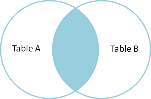

(Image from http://blog.codinghorror.com/a-visual-explanation-of-sql-joins/)

The inner join only includes data whose index appears in both tables. Let’s see what that looks like:

df_joined = df1.merge(df5, left_index=True, right_index=True)

df_joined

	area	population	mean temperature	elevation	annual rainfall	Mean House Price	median income	walkability score
London	4.898594	6.625739	3.587877	6.063331	4.342769	4.848734	6.598818	5.442444
Paris	6.032702	3.479265	2.383832	5.251509	5.158178	5.294294	4.282418	5.741057

Here, we have a couple of arguments specifying the manner of the join - we have specified that we are joining on the index of the left and right dataset with the optional “left_index=True” and “right_index=True”. Less obviously, the left dataset is df1 (because we’re using df1.merge() and the right dataset is df5 (because it appears as an argument in merge(). There’s no special reason it shouldn’t be the other way around, but for this function, it is this way around and we need to remember that when we use it.

Inner Space

Although we haven’t specified it, the merge() function has defaulted to an inner join (like the diagram above). We can specify how the join is calculated by changing the text in the optional argument “how”:

df_joined = df1.merge(df5, left_index=True, right_index=True, how='inner')

df_joined

	area	population	mean temperature	elevation	annual rainfall	Mean House Price	median income	walkability score
London	4.898594	6.625739	3.587877	6.063331	4.342769	4.848734	6.598818	5.442444
Paris	6.032702	3.479265	2.383832	5.251509	5.158178	5.294294	4.282418	5.741057

The Future of The Left

The left join includes all rows where the index appears on the left hand side of the join, and any data which matches it on the right hand side. If the index appears on the left but not the right, it will include the data from the left table, and have blanks for the columns on the right.

data_path = "https://s3.eu-west-2.amazonaws.com/qm2/wk3/left.png"
Image(data_path)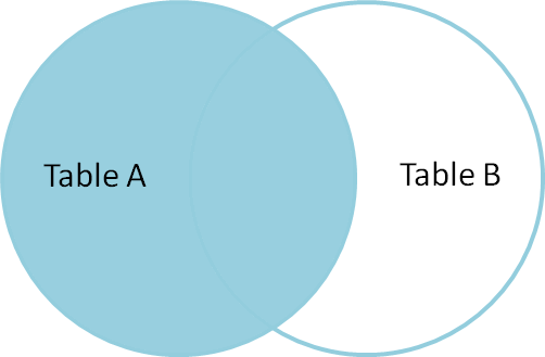

What does this look like? We will use the how=‘left’ optional argument to create a left join:

df_joined = df1.merge(df5, left_index=True, right_index=True, how='left')

df_joined

	area	population	mean temperature	elevation	annual rainfall	Mean House Price	median income	walkability score
London	4.898594	6.625739	3.587877	6.063331	4.342769	4.848734	6.598818	5.442444
Paris	6.032702	3.479265	2.383832	5.251509	5.158178	5.294294	4.282418	5.741057
Beijing	4.368419	4.993774	2.942992	3.761624	6.002863	NaN	NaN	NaN
Medellin	7.437921	5.228150	3.902431	4.437361	5.563400	NaN	NaN	NaN
Port Elizabeth	7.053265	5.936734	5.842155	6.042136	7.057592	NaN	NaN	NaN

As we see, the missing data appears as NaN - Not a Number.

Exercise:

Carry out right and outer joins on the dataframes df1 and df5 and explain how they’re filtering and joining the data.

I Am The One and Only

So far, we’ve carried out joins on data which have a one-to-one relationship; data for cities or people. What if our data has a one-to-many correspondence?

Example: We want to look at the quality of life in cities (a real student project from 2014). We have a dataset listing city-level characteristics for a number of cities in Europe, including the country each city is in. We also have a dataset listing the GDP, life expectancy and other indicators for a number of countries in Europe. How do we create a dataframe which, for each city, lists all of the characteristics of a city and those of its parent country?

We’ll be working now with data from the UN, covering information about cities - real data this time. The UN has some great data, we’ve taken some from here and processed it in various ways:

http://data.un.org/Data.aspx?d=POP&f=tableCode%3A240

Let’s load up data on city population - this set contains data for 2012-2014 inclusive:

data_path = "data/wk5/UN_Cities_1214_population.csv"

city_pop = pd.read_csv(data_path, encoding='latin1')

city_pop.head()

	Year	Area	Sex	City	City type	Record Type	Reliability	Source Year	Value	Value Footnotes
0	2013	Total	Both Sexes	MARIEHAMN	City proper	Estimate - de jure	Final figure, complete	2014	11370.0	NaN
1	2013	Total	Male	MARIEHAMN	City proper	Estimate - de jure	Final figure, complete	2014	5445.0	NaN
2	2013	Total	Female	MARIEHAMN	City proper	Estimate - de jure	Final figure, complete	2014	5925.0	NaN
3	2012	Total	Both Sexes	MARIEHAMN	City proper	Estimate - de jure	Final figure, complete	2013	11304.5	NaN
4	2012	Total	Male	MARIEHAMN	City proper	Estimate - de jure	Final figure, complete	2013	5408.0	NaN

Exercise

There is a another datafile we downloaded called UN_Cities_1214_country.csv. This is saved to data/wk5/UN_Cities_1214_country.csv - Load this into a dataframe called city_c with the city name as the index and view it; then, using merge on city name with city_pop to create a new dataframe called cities. You’ll probably get some errors. google the error messages, or ask ChatGPT/Gemini to help you understand them.

Hints: You’ll notice that the index won’t be the column you want to merge on in the city_pop data. What column should you merge on in city_pop? Which column should you merge on in city_c?

The syntax for merging on a column (which is not the index) is to pass the column name to the optional ‘left_on=’ or ‘right_on=’ arguments. And we don’t use right_index=True (or left_index=True), depending on which we’re using.

So for example: df1.merge(df2, left_on=‘Name’, right_index=True) would join df1 (on the left) to df2 (on the right), using the column ‘Name’ on the left (df1) and the index column (whatever that is) on the right (df2).

A footnote about footnotes

Just a quick note - if you look at the primary UN data, you’ll see footnotes which will confuse the hell out of Pandas. I’ve taken the footnotes out, but you can use .tail() to see whether there’s any junk in the trunk, and remove it via a text editor.

Clean data

We need to simplify this data a bit in the following ways:

1. I’m going to focus on one year (2012)
2. I’m going to just look at “Both Sexes” (not focus on one gender)
3. I’m going to get rid of a column of data (the ‘Value Footnotes’ column) using the drop() method.

cities = cities[cities['Sex']=='Both Sexes']
cities = cities[cities['Year']==2012]
cities.drop('Value Footnotes', axis=1, inplace=True)

NameError: ignored

cities.head()

Extension: In My Place

The command I used to get rid of that column is cities.drop(‘Value Footnotes’, axis=1, inplace=True). The syntax is not so complex - the first argument, ‘Value Footnotes’, is just the name of the column; the second argument, axis=1, tells Pandas to look for a column to remove (instead of a row which has axis=0); the third and final argument, inplace=True, is a command that tells Pandas to edit inplace, i.e. to edit the dataframe (cities) directly. When inplace is False (the default), this command does not directly edit cities, but instead provide an output. So the syntax for that would be

new_cities = cities.drop(‘Value Footnotes’, axis=1)

and new_cities would be a version of cities without the offending column. This is usually the safer option.

Life, Oh Life

The UN also has useful data by country, so let’s try and work with some of that and join it up with our city data. Let’s work with Life Expectancy Data:

http://data.un.org/Data.aspx?d=WDI&f=Indicator_Code%3ASP.DYN.LE00.IN

life = pd.read_csv('https://s3.eu-west-2.amazonaws.com/qm2/wk3/UN_Life_all.csv', index_col=0)

life.head()

Exercise:

In a new cell, clean up the above dataframe by

• removing the “Value Footnotes” Column
• use only the most recent data (2012)

Let’s make it a little clearer what “Value” refers to, by renaming the column. This is one way to do that:

life.rename(columns={'Value':'Life Expectancy'}, inplace=True)

life.head()

Now, merge this data with the cities data to show life expectancy for each city (based on the country it is in), and show the first 5 rows.

Plot population against life expectancy. Use plot’s optional arguments to specify the x column, y column, and that kind=‘scatter’.

Question: How much data was “missing” in the merge?